

1. Introduction
In this next series of posts, we move onto step 5, which is memorizing the TOOLS & TECHNIQUES associated with each process. In order to breakdown the memorizing into more bite-size chunks, I am going to break down this topic into 9 posts, one on each knowledge area.
This post covers chapter 7 of the PMBOK® Guide, which covers the Cost Knowledge Area. This knowledge area contains 3 processes, each of which has many techniques.
Here’s a description of the six processes that are included in the Cost Knowledge Area, together with a listing of the Tools & Techniques used in those processes.
| Process Name |
Process Description | Tools & Techniques |
| 7.1 Estimate Costs | Developing an approximation of the monetary resources needed to complete project activities. | 1. Expert judgment 2. Analogous estimating 3. Parametric estimating 4. Bottom-up estimating 5. Three-point estimating 6. Reserve analysis 7. Cost of quality 8. Project management estimating software 9. Vendor bid analysis
|
| 7.2 Determine Budget | Sums up the estimated costs and add reserves to establish an authorized cost baseline. | 1. Cost aggregation 2. Reserve analysis 3. Expert judgment 4. Historical relationships 5. Funding limit reconciliation
|
| 7.3 Control Costs | Monitoring the status of the project to update project budget and manage changes to the cost baseline. | 1. Earned value management 2. Forecasting 3. To-complete performance index (TCPI) 4. Performance reviews 5. Variance analysis 6. Project management software |
Let’s take a look at the tools & techniques for the 3 processes 7.1 through 7.3 in the Cost Knowledge Area.
7.1 ESTIMATE COSTS
7.1.1 Expert Judgment
Any time you are dealing with basics of the schedule and/or budget, it is vital to have expert judgment. Expert judgment can include being guided by historical information, either from within the company, or data that is publicly available.
7.1.2 Analogous estimating
Analogous estimating means estimating based on a previous similar project. It is a gross value approach, as opposed to parametric estimating (tool & technique 7.1.3). An example would be building a house in a subdivision where there are a limited number of models. If you are building a new house that is similar to one of the houses built before, you could do an analogous estimate by averaging the cost of constructing those houses that have been built before along a similar model plan.
Analogous estimating can be carried out by using tool & technique 6.4.1 (Expert Judgment and historical information).
NOTE: analogous estimating is less costly to carry out than other techniques, but it is also less accurate.
7.1.3 Parametric estimating
Parametric estimating means estimating based on some sort of activity parameter, such as cost, budget, and duration. An example using the construction of a house, as a contrast to the example given with the tool & technique of analogous estimating (7.1.2), would be estimating the cost of building a house by taking the average cost per square foot of constructing the previous homes in the subdivision.
This estimating technique is more accurate than analogous estimating.
7.1.4 Bottom-up estimating
This technique takes the estimates based on each work package, and then aggregates them “upward”, hence the title of bottom-up estimating. As opposed to top-down estimating methods like analogous estimating and parametric estimating (7.1.2 and 7.1.3), they are more costly to carry out but more accurate.
7.1.5 Three-point estimates
With this technique, you develop the following three estimates
|
Scenario |
Symbol |
Description |
| Most likely |
Tm |
The duration of the activity based on realistic expectations. |
| Optimistic |
To |
The activity duration based on the best-case scenario. |
| Pessimistic |
Tp |
The activity duration based on the worst-case scenario |
Then there are two three-point estimates that can be used, the simple average or the weighted average, also known as PERT.
Simple average = (To + Tm + Tp)/3
PERT = (To + 4Tm + Tp)/6
The number in the denominator is based on the number of terms in the numerator. If you remember that the PERT technique used an average that gives 4 times as much weight to the most likely scenario, then you can remember that the denominator is 6 rather than 3 for the simple average, because there are in effect 6 terms in the numerator and not 3.
7.1.6 Reserve analysis
If there is uncertainty in the schedule based on the probability of certain events occurring, i.e., risks, then these can be used to build contingency reserves. If an event occurs which would cost a certain amount x to handle, and that event has a probability of 10% occurring, then you would add a contingency reserve of 0.1x.
7.1.7 Cost of Quality (COQ)
The costs of conformance to quality standards (costs of preventing poor quality in the first place, plus costs for assessing the quality such as inspections) are outlined, and contrasted with the costs of nonconformance to quality standards (costs of correcting poor quality or dealing with customers who receive products with poor quality).
7.1.8 Project management estimating software
This is naturally a tool rather than a technique. Microsoft Project or Primavera are examples of software which can be used to help estimate costs.
7.1.9 Vendor Bid Analysis
If the project contains subprojects which are bid out to contractors, then there is a need to estimate the costs of that part of the project based on the bids submitted by contractors.
7.2 DETERMINE BUDGET
7.2.1. Cost aggregation
You take the WBS or Work Breakdown Structure which has the project broken down into work packages, which are further broken down into activities.
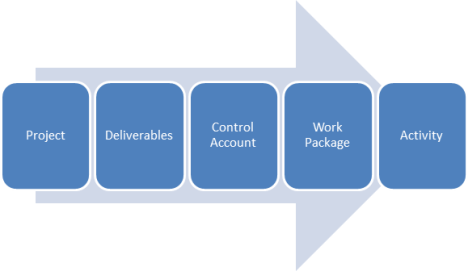
With cost aggregation, you basically go back the other way. See the steps in the figure below.
a. First you take the costs for each activity and summing them to get the costs for each work package.
b. Control accounts are basically placeholders in the work breakdown structure where you calculate all of the work packages below that level. They are put there in the Planning Process so you can see when the project is actually running and you are in the Monitoring & Controlling Process, you can take a snapshot of where you are, and see whether you are coming in under or overbudget. The next step is to sum up the work packages estimates in each control account to get the control account estimates.
c. Finally, you sum up the control account estimates, and you get the project estimate.
NOTE: THIS IS NOT THE SAME AS THE PROJECT BUDGET. To understand why this is so, see the next tool & technique 7.2.2 Reserve analysis.

7.2.2. Reserve analysis
Okay, so we’ve got the project estimate from the last tool & technique 7.2.1 Cost Aggregation. The process of risk analysis identifies what are essentially the “known unknowns,” i.e., what risks are planned for in terms of risk responses. The costs of responding to these risks through changes to the project scope and/or cost are the “contingency reserves.” The contingency reserves are added to the project estimate to get the cost baseline.
But, wait, there’s more! There are always the “unknown unknowns,” or risks which have NOT been accounted for in the risk register. Management reserves are the costs of unplanned changes to the project scope and/or cost. These are added to the cost baseline to get the cost budget.
NOTE: Here’s a short table comparing contingency reserves and management reserves, because these frequently became confused in our study sessions.
| Type of Reserves | Added to … | equals … | and is controlled by … |
| Contingency | Project estimate | Cost baseline | Project manager |
| Management | Cost baseline | Cost budget | Management (sponsors) |

7.2.3 Expert judgment
Any time you are dealing with basics of the schedule and/or budget, it is vital to have expert judgment. Expert judgment can include being guided by historical information, either from within the company, or data that is publicly available.
7.2.4 Historical relationships
If there is a similar project that was done in the past, this information can be used to develop a parametric or analogous estimate.
7.2.5 Funding limit reconciliation
The expenditure of funds for a project over the course of the project has to be recondiled with the funding limit for a project. It’s not a matter of just the total amount of funds; it is a cash-flow issue of how much money is available during each month of the project. The variance between the funding limit and the cost budget for the project during each time period (month, quarter, or whatever) needs to be reconciled. If the cost budget exceeds the funding limit for a particular period, work may have to be rescheduled in order to level out the rate of expenditures. This is similar to the resource leveling technique.
7.3 CONTROL COSTS
7.3.1. Earned value management
Earned value management can answer the question “where are we now in relationship to the budget?”. The values of Cost Variance (CV) = Earned Value (EV) – Actual Costs (AC) or alternatively, the Cost Performance Index (CPI) = Earned Value (EV) / Actual Costs (AC). A positive CV is good and a negative CV is bad; a CPI > 1 is good, and a CPI < 1 is bad.
7.3.2. Forecasting
Forecasting can answer the question “given where we are now (which was determined with the tool and technique of 7.3.1 Earned value management), where will we be by the end of the project in relationship to the budget?”
To do forecasting, you need to know the Budget at Completion or BAC, the Estimate at Completion (EAC), the Estimate to Complete or (ETC), and the Variance at Completion or (VAC). Here are the definitions of these terms.
| Quantity | Formula | Definition |
| Budget at Completion (BAC) | (Related to PV) | Authorized budget amount of the total project, i.e. what the project was supposed to cost |
| Estimate at Completion (EAC) | (several formulas) | Estimated cost of the project at completion, i.e., what the project is now expected to cost |
| Variance at Completion (VAC) |
BAC – EAC | The difference between what the project was supposed to cost (BAC) and what is now expected to cost (EAC). |
| Estimate to Complete | EAC – AC | How much more it is estimated it will cost to complete the project, i.e., the difference between what the total project is now expected to cost (EAC) and how much it has cost until now (AC). |
How are they related? Look at the following schematic.
BAC or the Budget at Completion is where the budget is planned to be at the end of the budget, i.e., the total cost budget. The EAC is the estimate of where the budget will be IF the costs keep going as they have up until now, as given by the AC or Actual Costs. The additional amount of money it is estimated to take you from now until the end of the project is the ETC or Estimate to Complete. You can see by the relationships below that by definition, ETC = EAC – AC. Another term is the difference between what the project was supposed to cost (BAC) and what is now expected to cost (EAC), and this is the VAC or Variance at Completion, and by definition, VAC = BAC – EAC.
| Project | START |
NOW |
END |
|||
| Planned | ß |
PV |
à |
|||
| ß | BAC |
à |
||||
| Actual | ß |
AC |
à |
|||
| Estimate |
ß | EAC |
à |
|||
| ß |
ETC |
à |
||||
| ßVACà | ||||||
How do you calculate EAC? Here’s the trick: there are 4 ways to calculate it depending on why your actual costs (AC) are at variance from the budget.
|
Formula No. |
Formula |
Formula Name |
Formula Explanation |
|
1 |
EAC = AC + ETC |
New estimate |
ETC is new bottom-up estimate |
|
2 |
EAC = AC + (BAC – EV) |
Original estimate |
Reason for variance is one-time occurrence |
|
3 |
EAC = AC + (BAC – EV)/CPI Or EAC = BAC/CPI
|
Performance estimate low |
Reason for variance will continue at same rate |
|
4 |
EAC = AC + (BAC – EV)/CPI*SPI |
Performance estimate high |
Reason for variance will continue and effect performance |
Formula 1.
EAC = AC + (ETC)
If the original budget is considered totally flawed, or you have no idea why there is such a large variance, then one way to estimate the amount it will now take to do the project is to take the amount spent on the project so far (AC) and then do a more accurate bottom-up estimate of the amount it will take to complete the project (ETC). That’s essentially saying that you have to refigure the budget from scratch starting from now until the end of the project.
Formulas 2-4. The rest of the formulas are similar in that they all start with AC, the actual cost up to now, and then they add an amount called the remaining costs or BAC – EV, modified by some other factor.
Formula 2.
EAC = AC + (BAC – EV)
If the reason for the variance is a one-time occurrence, we don’t expect that it will happen again. Then you just take the remaining costs or (BAC – EV) and add them to what the project has already cost to get the estimate at completion of EAC. Picture the budget as a straight road going from one town to another. The variance is a one-time thing that causes the budget to suddenly vary by a small amount, as if you were driving a car and a sudden gust of wind caused your car to be blown a few feet into another lane, but then your car continues along a straight line to the other side.
Formula 3.
EAC = AC + (BAC – EV) / CPI = BAC/CPI
If the reason for the cost variance is a continuing occurrence, then you take your actual costs and add it to the remaining costs or (BAC – EV) divided by the current cost performance index (CPI). The algebra allows this expression to be simplified to the planned budget amount or BAC divided by the current cost performance index or CPI.
In the analogy of driving a car, let’s say you take a wrong turn onto a road which is going at a certain angle to the road you are driving on. This formula assumes that you are continuing on that same wrong road until you get to the destination.
Formula 4. S
EAC = AC + (BAC – EV)/(CPI * SPI)
If the reason for the cost variance is a continuing occurrence which also effects the schedule variance, you take your actual costs and add it to the remaining costs or (BAC – EV) divided by BOTH the current cost performance index (CPI) and the schedule performance index (SPI).
In the analogy of driving a car, let’s say you take a wrong turn onto a road which is not going at a certain specified angle to the road you are driving on, but is actually curving away from that road. This formula assumes that you are continuing on that same wrong that is curving away from the first road (budget) until you get to the destination.
7.3.3. To-complete performance index (TCPI)
The To-complete performance index or TCPI can answer the question “given where we are now, how fast to we have to go to be within budget by the end of the project?”
Okay, here’s an analogy to tell you how this works. Let’s say you are driving from city A to city B which takes 6 hours normally. You have calculated that you can drive there if you go at the speed limit of 65 mph for the entire trip. You get halfway there and you do a quick calculation which tells you that you have actually only gone an average of 55 mph. How fast will you have to go to make it to your destination on the second half of your trip in the same time frame of 6 hours? Well, the answer is 75 mph. This will increase the risk of getting a speeding ticket, of course.
In a similar way, if your CPI is below 1, then the TCPI will end up giving you an index that is greater than 1, because if you are over budget so far, you will have to be UNDER budget for the rest of the project to make up for the overage you have had so far.
Here is the formula for TCPI:
TCPI = (BAC – EV)/(EAC – AC).
Memorizing this formula is not as crucial as memorizing the other formulas related to earned value management; however, it is important to understand the CONCEPT behind it.
7.3.4. Performance reviews
This measures the performance of the project compared to the cost baseline, i.e., the budget.
7.3.5. Variance analysis
Using the results of the performance reviews (see the previous tool 7.3.4), earned value analysis can be used to calculate cost variance (CV) or the cost performance index (CPI).
7.3.6. Project management software
Project management software such as Microsoft Project or Primavera can be used to track what your actual costs are compared to where your costs are supposed to be according to the budget.
The next post will be on the Tools & Techniques associated with chapter 8, the Quality Knowledge Area.
Filed under: Uncategorized |

Leave a comment