

1. Introduction
In this next series of posts, we move onto step 5, which is memorizing the TOOLS & TECHNIQUES associated with each process. In order to breakdown the memorizing into more bite-size chunks, I am going to break down this topic into 9 posts, one on each knowledge area.
This post covers chapter 6 of the PMBOK® Guide, which covers the Time Knowledge Area. However, since this knowledge area contains 6 processes, each of which has many techniques, I have decided to divide this material into two posts. This is the second part, which covers the last 3 of these 6 processes.

Here’s a description of the six processes that are included in the Time Knowledge Area, together with a listing of the Tools & Techniques used in those processes. As a reminder, this post will cover only 6.4 through 6.6 of the tools and techniques, but I’m including all six processes in this chart for the sake of completeness.
| Process Name |
Process Description | Tools & Techniques |
| 6.1 Define Activities | Identifying actions to be performed to produce product deliverables. | 1. Decomposition 2. Rolling wave planning 3. Templates 4. Expert judgment
|
| 6.2 Sequence Activities | Identifying and documenting relationships among the project activities. | 1. Precedence diagramming method (PDM) 2. Dependencey determination 3. Applying leads and lags 4. Schedule network templates
|
| 6.3 Estimate Activity Resources | Estimating type and quantities of resources (human and material) required to perform each activity. | 1. Expert judgment 2. Alternatives analysis 3. Published estimating data 4. Bottom-up estimating 5. Project management software |
| 6.4 Estimate Activity Durations | Approximating the number of work periods needed to complete individual activities with estimated resources. | 1. Expert judgment 2. Analogous estimating 3. Parametric estimating 4. Three-point estimates 5. Reserve analysis
|
| 6.5 Develop Schedule | Analyzing activity sequences, durations, resources requirements, and schedule constraints to create product schedule. | 1. Schedule network analysis 2. Critical path method 3. Critical chain method 4. Resource leveling 5. What-if scenario analysis 6. Applying leads and lags 7. Schedule compression 8. Scheduling tool
|
| 6.6 Control Schedule | Monitoring the status of the project to update project progress and manage changes to schedule baseline. | 1. Performance reviews 2. Variance analysis 3. Project management software 4. Resource leveling 5. What-if scenario analysis 6. Adjusting leads and lags 7. Schedule compression 8. Scheduling tool |
Let’s take a look at the tools & techniques for processes 6.4 through 6.6 in the Time Knowledge Area.
6.4 ESTIMATE ACTIVITY DURATIONS
6.4.1 Expert Judgment
Any time you are dealing with basics of the schedule and/or budget, it is vital to have expert judgment. Remember that, when it comes to figuring out how long it will take to complete the work, one of the first experts you should consult is the person who is doing the work, especially if they have done that work before in the past. Expert judgment can include being guided by historical information, either from within the company, or data that is publicly available.
6.4.2 Analogous estimating
Analogous estimating means estimating based on a previous similar project. It is a gross value approach, as opposed to parametric estimating (tool & technique 6.4.3). An example would be building a house in a subdivision where there are a limited number of models. If you are building a new house that is similar to one of the houses built before, you could do an analogous estimate by averaging the cost of constructing those houses that have been built before along a similar model plan.
Analogous estimating can be carried out by using tool & technique 6.4.1 (Expert Judgment and historical information).
NOTE: analogous estimating is less costly than other techniques, but it is also less accurate.
6.4.3 Parametric estimating
Parametric estimating means estimating based on some sort of activity parameter, such as cost, budget, and duration. An example using the construction of a house, as a contrast to the example given with the tool & technique (6.4.2), would be estimating the cost of building a house by taking the average cost per square foot of constructing the previous homes in the subdivision.
This estimating technique is more accurate than analogous estimating.
6.4.4 Three-point estimates
With this technique, you develop the following three estimates
|
Scenario |
Symbol |
Description |
| Most likely |
Tm |
The duration of the activity based on realistic expectations. |
| Optimistic |
To |
The activity duration based on the best-case scenario. |
| Pessimistic |
Tp |
The activity duration based on the worst-case scenario |
Then there are two three-point estimates that can be used, the simple average or the weighted average, also known as PERT.
Simple average = (To + Tm + Tp)/3
PERT = (To + 4Tm + Tp)/6
The number in the denominator is based on the number of terms in the numerator. If you remember that the PERT technique used an average that gives 4 times as much weight to the most likely scenario, then you can remember that the denominator is 6 rather than 3 for the simple average, because there are in effect 6 terms in the numerator and not 3.
6.4.5 Reserve analysis
If there is uncertainty in the schedule based on the probability of certain events occurring, i.e., risks, then these can be used to build contingency reserves. If an event occurs which would cost a certain amount x to handle, and that event has a probability of 10% occurring, then you would add a contingency reserve of 0.1x.
6.5 DEVELOP SCHEDULE
6.5.1. Schedule network analysis
Schedule network analysis is the collection of tools and techniques you use to generate the project schedule. These include technique 6.5.2 Critical Path method, 6.5.3 Critical chain method, 6.5.4 Resource leveling, and 6.5.5 What-if scenario analysis.
The schedule is then further refined using technique 6.5.6 Applying leads and lags and 6.5.7 Schedule compression. The software sometimes used to carry out these techniques is the tool 6.5.8 Scheduling tool.
6.5.2. Critical path method
To determine how long a project will take, you need to find out the critical path, that is, the sequence of activities in the network diagram that is the longest. Other paths along the network will yield sequences of activities that are shorter than the critical path, and they are shorter by an amount equal to the float. This means that activities that have float could be delayed by a certain amount without affecting the schedule. Activities along the critical path have a float of zero. This means that any delay along the critical path will affect the schedule.
Here’s an outline of the critical path methodology.
a. You create a network diagram of all the activities.
b. You label each activity with the duration derived from process 6.4 Estimate Activity Durations.
c. You do a forward pass to determine the early start and early finish date of all activities, from the start of the project to the end of the project.
d. Once at the end of the project, you do a backward pass to determine the late start and late finish date of all activities, from the end of the project to the start of the project.
e. For each activity, you use the results of c and d to calculate the float of each activity.
f. All activities that have 0 float are on the critical
path for that project.
Let’s take a look at the methodlogy in general.
Step 1. For each activity, create a matrix which will contain the duration, the early start, the early finish, the late start, late finish, and float for a particular activity.
|
Activity Number |
|
|
Duration |
|
| Early Start (ES) | Early Finish (EF) |
| Late Start (LS) | Late Finish (LF) |
|
Float |
|
Here are the meanings of the numbers in the boxes:
Activity Number: you can label them A through Z, or 1 through N, just as long as each activity has a unique identifier.
Duration: this is the number that you should get as an output of the 6.4 Estimate Activity Durations process.
Early Start (ES): The Early Start is the number you begin the analysis with to do the forward pass. It is defined as 0 for the first activity in the project. The Early Start for subsequent activities is calculated in one of two different ways, which will be demonstrated below.
Early Finish (EF): This is the next number you go to in the forward pass analysis. It is taken by adding the number in the ES box plus the number in the Duration box.
Late Finish (LF): The Late Finish is the number you begin the analysis with to do the backward pass. It is defined to be equal to the number in the Early Finish box for the last activity in the project. The Late Finish for preceding activities is calculated in one of two different ways, which will be demonstrated below.
Late Start (LS): This is the next number you go to in the backward pass analysis. It is taken by subtracting the number in the Duration box from the number in the LF box.
Float: Once ES, ES, LF, and LS are determined, the float is calculated by either LS – ES or LF – EF. Just remember that a piece of wood will float to the top of the water, so the float is calculated by taking the bottom number and then going upward and subtracting the number that’s on the top of it.
Step 2.
For activity A, the first activity in the project, ES = 0.
|
A |
|
|
0 |
|
Step 3.
Then EF for activity A is simply ES + duration. Let’s say activity A takes 5 days. Then EF = 0 + 5 = 5.
|
A |
|
|
5 |
|
|
0 |
5 |
Step 4.
The forward pass for activity A is complete. Let’s go on to activity B.

Since activity B has only one predecessor, activity B, the ES for activity B is simply equal to the EF of activity A, which was 5.
|
B |
|
|
3 |
|
|
5 |
|
Then the EF for activity B is taken by adding the ES of to the duration of activity B or 3, giving EF = 5 + 3 = 8.
There’s one more situation that we have to discuss and that is if an activity has more than one predecessor.
Let’s assume the durations for each activity are as follows:
| Activity | Duration |
| A | 5 |
| B | 3 |
| C | 6 |
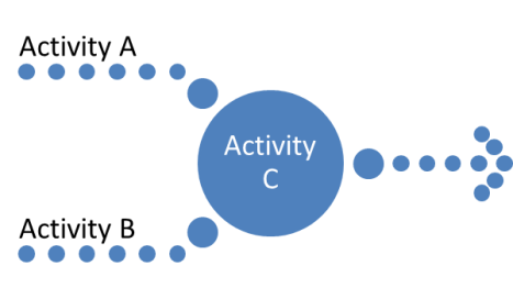
Assume Activity A and Activity B are both done concurrently at the start of the project, and both need to be done in order for Activity C to start. Well, before we do the formal forward pass analysis, what does logic tell us. Activity A takes 5 days; Activity B takes 3 days. Both activity A and B have to be done before Activity C can take place. In this case the start date of the project is considered to be 0. Can Activity C take place on day 3, when activity B is done? No, because Activity A isn’t completed yet, and you need BOTH A and B to be done. The earliest possible start date for Activity C will be day 5, because only on that date will both A and B be done.
So this illustrates the other way of calculating ES for an activity B. If there are multiple predecessors, then the ES is equal to the LARGEST of the ES of the predecessor activities.
Step 5.
Now, let’s assume we are at the end of the project at activity Z.
|
Z |
|
|
5 |
|
|
95 |
100 |
EL = ES + duration gives us EL = 95 + 5 + 100. So the project will take 100 days according to our forward pass calculation.
Now, we have the backward pass.
We start this out by stating as a principle that the late finish or LF date for the last activity in the project is equal to the EF date.
|
Z |
|
|
5 |
|
|
95 |
100 |
|
100 |
|
Then, of course, the late start date or LS = LF – duration = 100 – 5 = 95.
|
Z |
|
|
5 |
|
|
95 |
100 |
|
95 |
100 |
Step 6.
Now we go in the reverse direction towards the beginning of the network diagram, this time filling out the bottom LS and LF boxes for each activity.
If the activity has one successor, then the LF for the predecessor activity equals the LS for the successor of activity. But if there are more than one predecessor activity, then here’s what you do. For the forward pass, you take the highest EF of all predecessors.
For the backward pass, you take the lowest LS of all successors. Let’s see how this works.

Let’s assume the forward pass is done on A, B, and C. We do the backward analysis and we get to the following point. What is the LF of activity A?
|
A |
B |
C |
|||
|
5 |
3 |
4 |
|||
|
0 |
5 |
5 |
8 |
5 |
9 |
|
6 |
9 |
5 |
9 |
||
Well, activity B and activity C are both successors of A. In this case, activity B has an LS of 6 and activity C has an LS of 5. The earliest LS is therefore 5, and so LS of activity A is 5.
|
A |
B |
C |
|||
|
5 |
3 |
4 |
|||
|
0 |
5 |
5 |
8 |
5 |
9 |
|
0 |
5 |
6 |
9 |
5 |
9 |
Step 7.
What is the float? Take LF – EF (or LS – ES) for each of the activities.
|
A |
B |
C |
|||
|
5 |
3 |
4 |
|||
|
0 |
5 |
5 |
8 |
5 |
9 |
|
0 |
5 |
6 |
9 |
5 |
9 |
|
0 |
1 |
0 |
|||
So the float of B is 1, and the float of A and C are 0. Therefore A and C are on the critical path.
6.5.3. Critical chain method
The critical chain method takes the critical path method and adds an element of resource leveling. Okay, so you’ve found the critical path according to the critical path methodology in technique 6.5.2 Critical path method. You modify the resources based on resource leveling¸ which is described in the next section below.) You need to adjust the schedule to reflect this. This may, in turn, alter the critical paths done with the technique 6.5.2 Critical path method.
The result is a modified version of the network diagram and perhaps a new critical path.
6.5.4. Resource leveling
Let’s say that the activity requires 4 days, consisting of 4 people working 8 hours a day. But let’s say that these people are working on two different projects, and each is available for only 4 hours a day. That means in reality the project will take 8 days. Using a resource histogram, or a bar chart which shows how much each person can work on the project during the day, you may have to adjust your activity durations to reflect the reality of the human resources available. The results of resource leveling are used to adjust the critical path in technique 6.5.3 Critical chain method.
6.5.5. What-if scenario analysis
This is essentially risk analysis applied to the network analysis, meaning that you look out for adverse conditions that may impact the project. Of course, you can also look for favorable conditions that may impact the project. These give you the basis for the optimistic and pessimistic projections of activity durations. Calculating the probability of multiple project durations is called a Monte Carlo Analysis. This gives a distribution of possible outcomes for the total project, rather than a simple optimistic and pessimistic outcome.
6.5.6. Applying leads and lags
If an activity is required to be delayed or accelerated, then this is used to further refine the network analysis, and could possibly alter the critical path as found out in the 6.5.2 Critical Path Method.
6.5.7. Schedule compression
There are two methods for shortening the project schedule without changing the project scope. However, they may increase other constraints, such as cost and risk.
|
Method |
Description |
|
Crashing |
Reduction of activity duration by adding resources, i.e., paying for additional staff to do the work. This increases the cost. |
|
Fast Tracking |
Taking activities normally done in series, i.e., one after the other, and doing them in parallel, so that they overlap. This increases the risk. |
6.5.8. Scheduling tool
This is essentially scheduling software such as Microsoft Project or Primavera.
6.6 CONTROL SCHEDULE
Many of the tools & techniques listed here have already been introduced as part of process 6.5 Develop Schedule. Except here rather than developing the schedule, they are being used to get the schedule back on track.
6.6.1. Performance reviews
This measures the performance of the project compared to the schedule baseline.
6.6.2. Variance analysis
Using the results of the performance reviews (see the previous tool 6.6.1), earned value analysis can be used to calculate schedule variance (SV) or the schedule performance index (SPI).
6.6.3. Project management software
Project management software such as Microsoft Project or Primavera can be used to track where you are compared to where you are supposed to be on the schedule.
6.6.4. Resource leveling
This was already described as technique 6.5.4, and it is used to optimize the distribution of work among resources to get the greatest effectiveness out of them.
6.6.5. What-if scenario analysis
This was already described as technique 6.5.5, and is used to review various possible scenarios that could occur that might affect the project in order to bring the schedule back into alignment with the plan.
6.6.6. Adjusting leads and lags
This was already described as technique 6.5.6, and is used to help bring the schedule back into alignment with the plan.
6.6.7. Schedule compression
This was already described as technique 6.5.7, and is used to help bring the schedule back into alignment with the plan.
6.6.8. Scheduling tool
Project management software such as Microsoft Project or Primavera includes a scheduling tool to generate a project schedule update.
The next post will be on the Tools & Techniques associated with chapter 7, the Cost Knowledge Area.
Filed under: Uncategorized |

Leave a comment